Usage and installation of shinyChromosome

This is the repository for the Shiny application presented in “shinyChromosome: An R/Shiny Application for Interactive Creation of Non-circular Plots of Whole Genomes” (Yu et al. Genomics Proteomics Bioinformatics. 2020).

Use shinyChromosome online

shinyChromosome is deployed at http://venyao.xyz/shinyChromosome/, http://shinychromosome.ncpgr.cn/ and https://yimingyu.shinyapps.io/shinychromosome/ for online use.
shinyChromosome is idle until you activate it by accessing the URLs.
So, it may take some time when you access this URL for the first time.
Once it was activated, shinyChromosome could be used smoothly and easily.

Launch shinyChromosome directly from R and GitHub

User can choose to run shinyChromosome installed on local computers (Windows, Mac or Linux) for a more preferable experience.

Step 1: Install R and RStudio

Before running the app you will need to have R and RStudio installed (tested with R 3.5.0 and RStudio 1.1.419).
Please check CRAN (https://cran.r-project.org/) for the installation of R.
Please check https://www.rstudio.com/ for the installation of RStudio.

Step 2: Install the R Shiny package and other packages required by shinyChromosome

Start an R session using RStudio and run these lines:

# try an http CRAN mirror if https CRAN mirror doesn't work
install.packages("shiny")
install.packages("rlang")
install.packages("zip")
install.packages("ggplot2")
install.packages("plyr")
install.packages("ggthemes")
install.packages("RLumShiny")
install.packages("RColorBrewer")
install.packages("gridExtra")
install.packages("reshape2")
install.packages("data.table")
install.packages("shinythemes")
install.packages("shinyBS")
install.packages("markdown")
# install shinysky  
install.packages("devtools")  
devtools::install_github("venyao/ShinySky", force=TRUE)  

Step 3: Start the app

Start an R session using RStudio and run these lines:

shiny::runGitHub("shinyChromosome", "venyao")  

This command will download the code of shinyChromosome from GitHub to a temporary directory of your computer and then launch the shinyChromosome app in the web browser. Once the web browser was closed, the downloaded code of shinyChromosome would be deleted from your computer. Next time when you run this command in RStudio, it will download the source code of shinyChromosome from GitHub to a temporary directory again. This process is frustrating since it takes some time to download the code of shinyChromosome from GitHub.

Users are suggested to download the source code of shinyChromosome from GitHub to a fixed directory of your computer, such as 'E:\apps' on Windows. Following the procedure illustrated in the following figure, a zip file named 'shinyChromosome-master.zip' would be downloaded to the disk of your computer. Move this file to 'E:\apps' and unzip this file. Then a directory named 'shinyChromosome-master' would be generated in 'E:\apps'. The scripts 'server.R' and 'ui.R' could be found in 'E:\apps\shinyChromosome-master'.

Then you can start the shinyChromosome app by running these lines in RStudio.

library(shiny)
runApp("E:/apps/shinyChromosome-master", launch.browser = TRUE)

Deploy shinyChromosome on local or web Linux server

Step 1: Install R

Please check CRAN (https://cran.r-project.org/) for the installation of R.

Step 2: Install the R Shiny package and other packages required by shinyChromosome

Start an R session and run these lines in R:

# try an http CRAN mirror if https CRAN mirror doesn't work  
install.packages("shiny")
install.packages("rlang")
install.packages("zip")
install.packages("ggplot2")
install.packages("plyr")
install.packages("ggthemes")
install.packages("RLumShiny")
install.packages("RColorBrewer")
install.packages("gridExtra")
install.packages("reshape2")
install.packages("data.table")
install.packages("shinythemes")
install.packages("shinyBS")
install.packages("markdown")
# install shinysky  
install.packages("devtools")  
devtools::install_github("venyao/ShinySky", force=TRUE)  

For more information, please check the following pages:
https://cran.r-project.org/web/packages/shiny/index.html
https://github.com/rstudio/shiny
https://shiny.rstudio.com/

Step 3: Install Shiny-Server

Please check the following pages for the installation of shiny-server.
https://www.rstudio.com/products/shiny/download-server/
https://github.com/rstudio/shiny-server/wiki/Building-Shiny-Server-from-Source

Step 4: Upload files of shinyChromosome

Put the directory containing the code and data of shinyChromosome to /srv/shiny-server.

Step 5: Configure shiny server (/etc/shiny-server/shiny-server.conf)

# Define the user to spawn R Shiny processes
run_as shiny;

# Define a top-level server which will listen on a port
server {  
  # Use port 3838  
  listen 3838;  
  # Define the location available at the base URL  
  location /shinychromosome {  
    # Directory containing the code and data of shinyChromosome  
    app_dir /srv/shiny-server/shinyChromosome;  
    # Directory to store the log files  
    log_dir /var/log/shiny-server;  
  }  
}  

Step 6: Change the owner of the shinyChromosome directory

$ chown -R shiny /srv/shiny-server/shinyChromosome  

Step 7: Start Shiny-Server

$ start shiny-server  

Now, the shinyChromosome app is available at http://IPAddressOfTheServer:3838/shinyChromosome/.

Input data format

The detailed format of input data for different types of plots are described in the following sections.

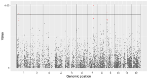
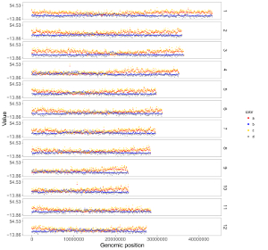
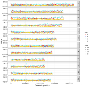
1. Single-genome plot

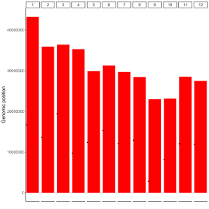
1.1 Genome data

The dataset should contain only 2 columns with fixed order. Column names are optional.
1st column: chromosome ID.
2nd column: chromosome length.

Acceptable input data format can be

 chr     size
   1 43268879
   2 35930381
   3 36406689

or

1   43268879
2   35930381
3   36406689

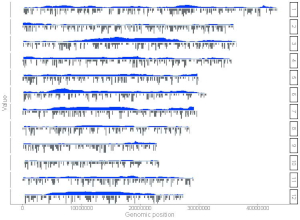
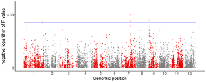
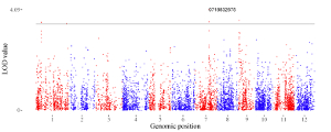
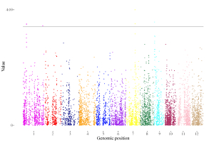
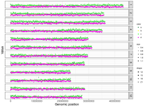
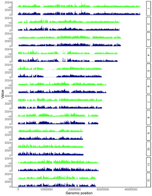
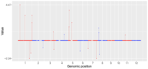
1.2 Point

The dataset should contain >=3 columns.
In the simplest situation, the dataset should contain 3 columns with fixed order. In this case, column names are optional.
1st column: chromosome ID.
2nd column: chromosome position.
3rd column: data value.

Acceptable input data format can be

 chr position    value
   1   202360 0.315323
   1   213775 1.113439
   1   218457 0.393112

or

1   202360  0.315323
1   213775  1.113439
1   218457  0.393112

To control the color of points, add a color column to categorize the data into different groups. Then different colors will be assigned to different groups of data. In this case, column names are compulsory. The name of the first three columns can be any appropriate variable names in R and the order of the first three columns must be fixed as the simplest situation. The name of the color column must be 'color'.

 chr position    value color
   1   202360 0.315323     a
   1   213775 1.113439     a
   1   218457 0.393112     a

To control the symbol used for each point, add a shape column. Check http://www.endmemo.com/program/R/pchsymbols.php for more information. In this case, column names are compulsory. The name of the first three columns can be any appropriate variable names in R and the order of the first three columns must be fixed as the simplest situation. The name of the shape column must be 'shape'.

 chr position value shape
   1        1    29    15
   1   100001    18    15
   1   200001    22    15

To control the size of each point, add a size column. Larger number in the size column means lareger point size. In this case, column names are compulsory. The name of the first three columns can be any appropriate variable names in R and the order of the first three columns must be fixed as the simplest situation. The name of the size column must be 'size'.

 chr position value size
   1        1    29  1.1
   1   100001    18  1.0
   1   200001    22  1.1

Users can choose to control two or more of the color, shape and size features at the same time. In this case, column names are compulsory. The name of the first three columns can be any appropriate variable names in R and the order of the first three columns must be fixed as the simplest situation. The name of the shape column must be 'shape'. The name of the color column must be 'color'. The name of the size column must be 'size'. The order of the color, shape and size columns is flexible. Acceptable input data can be

 chr position value color shape
   1        1    29     a    15
   1   100001    18     a    15
   1   200001    22     a    15

or

 chr position value color shape size
   1        1    29     a    15  1.1
   1   100001    18     a    15  1.0
   1   200001    22     a    15  1.1

or

 chr position value color size
   1        1    29     a  1.1
   1   100001    18     a  1.0
   1   200001    22     a  1.1

or

 chr position value shape size
   1        1    29    15  1.1
   1   100001    18    15  1.0
   1   200001    22    15  1.1

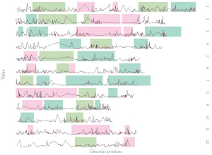
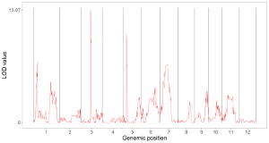
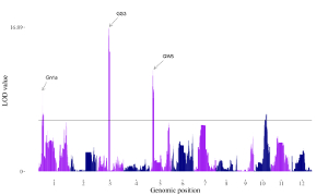
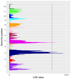
1.3 Line

The dataset should contain >=3 columns.
In the simplest situation, the dataset should contain 3 columns with fixed order. In this case, column names are optional.
1st column: chromosome ID.
2nd column: chromosome position.
3rd column: data value.

Acceptable input data format can be

 chr position  value
   1        0 0.0428
   1   565000 0.0522
   1   599000 0.0674

or

1        0  0.0428
1   565000  0.0522
1   599000  0.0674

To add multiple lines and assign different colors to different lines, add a color column to categorize the data into different groups. In this case, column names are compulsory. The name of the first three columns can be any appropriate variable names in R and the order of the first three columns must be fixed as the simplest situation. The name of the color column must be 'color'.

 chr position value color
   1        1    29     a
   1   100001    18     a
   1        1     4     b
   1   200001     5     b

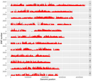
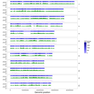
1.4 Bar

The dataset should contain >=4 columns.
In the simplest situation, the dataset should contain 4 columns with fixed order. In this case, column names are optional.
1st column: chromosome ID.
2nd column: start coordinate of bars.
3rd column: end coordinate of bars.
4th column: data value.

Acceptable input data format can be

 chr  start    end value
   1      1 100000   672
   1 100001 200000   486
   1 200001 300000   650

or

1        1  100000  672
1   100001  200000  486
1   200001  300000  650

To control the color of bars, add a color column to categorize the data into different groups. Then different colors will be assigned to different groups of data. In this case, column names are compulsory. The name of the first four columns can be any appropriate variable names in R and the order of the first four columns must be fixed as the simplest situation. The name of the color column must be 'color'.

 chr  start    end  value color
   1      0 565000 0.5923     a
   1 565000 599000 0.6701     a
   1 599000 922000 0.6785     a

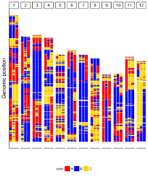
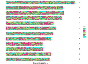
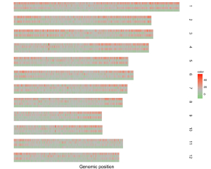
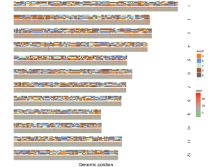
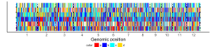
1.5 Rect

The dataset should contain 4 columns with fixed order. Column names are optional.
1st column: chromosome ID.
2nd column: start coordinate of rects.
3rd column: end coordinate of rects.
4th column: data value.

The 4th column can be a character vector or a numeric vector. For a character vector, choose the rect_discrete plot type. For a numeric vector, choose the rect_gradual plot type.

Acceptable input data format can be

 chr  start    end color
   1      1 100000     A
   1 100001 200000     C
   1 200001 300000     A

or

1        1  100000  A
1   100001  200000  C
1   200001  300000  A

or

 chr  start    end NTE
   1      1 100000  29
   1 100001 200000  18
   1 200001 300000  22

or

1        1  100000  29
1   100001  200000  18
1   200001  300000  22

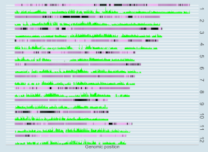
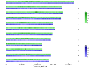
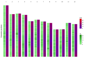
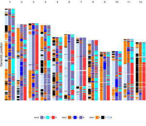
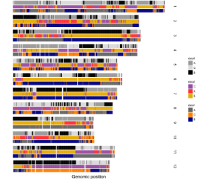
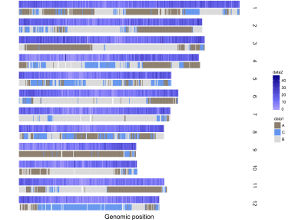
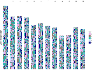
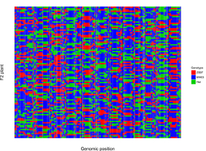
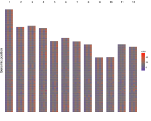
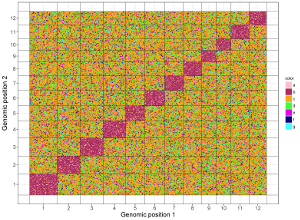
1.6 Heatmap

The dataset should contain >=4 columns. Column names are optional. The order of the first three columns must be fixed as follows.
1st column: chromosome ID.
2nd column: start coordinate of cells.
3rd column: end coordinate of cells.

Except for the first three columns, all the rest columns are treated as data values by shinyChromosome.
The rest columns can be character vectors or numeric vectors. Mix of character vector and numeric vector are not allowed.
For character vectors, choose the heatmap_discrete plot type. For numeric vectors, choose the heatmap_gradual plot type.

Acceptable input data format can be

 chr   start     end val1 val2 val3 val4 val5 val6
   1       0  631164    a    e    c    c    a    b
   1  631165 1749192    b    b    c    d    d    c
   1 1749193 2077793    c    e    a    b    e    e

or

1         0  631164 a   e   c   c   a   b
1    631165 1749192 b   b   c   d   d   c
1   1749193 2077793 c   e   a   b   e   e

or

 chr    start      end TE NTE TR NTR
   1        1   100000  4  29 17  45
   1 10000001 10100000  9  14 20  28
   1  1000001  1100000  1  16 -5  29

or

1          1      100000    4   29  17  45
1   10000001    10100000    9   14  20  28
1    1000001     1100000    1   16  -5  29

1.7 Segment

The dataset should contain 5 columns with fixed order. Column names are optional.
1st column: chromosome ID.
2nd column: X-axis start coordinate of segments.
3rd column: Y-axis start coordinate of segments.
4th column: X-axis end coordinate of segments.
5th column: Y-axis end coordinate of segments.

Acceptable input data format can be

 chr   xstart ystart     xend yend
   1   134291      0   134291  2.8
   1  2665412      0  2665412  2.8
   1 24392841      0 24392841  2.8

or

1     134291    0     134291    2.8
1    2665412    0    2665412    2.8
1   24392841    0   24392841    2.8

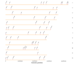
1.8 Text

The dataset should contain 4 columns with fixed order. Column names are optional.
1st column: chromosome ID.
2nd column: X-axis position of texts.
3rd column: Y-axis position of texts.
4th column: the symbols of texts.

Acceptable input data format can be

 chr     xpos ypos  symbol
   1   134291    3 OsTLP27
   1  2665412    3    MT2D
   1 24392841    3   OCPI1

or

1     134291    3   OsTLP27
1    2665412    3      MT2D
1   24392841    3     OCPI1

1.9 Vertical line

The dataset should contain 2 columns with fixed order. Column names are optional.
1st column: chromosome ID.
2nd column: genomic position of vertical lines.

Acceptable input data format can be

 chr position
   1        0
   1 43268879
   2 35930381

or

1          0
1   43268879
2   35930381

1.10 Horizontal line

The dataset should contain 1 column. Column names are optional.
1st column: Y-axis value of horizontal lines.

Acceptable input data format can be

 position
        8
       12
        5

or

 8
12
 5

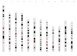
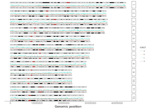
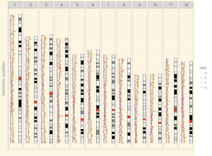
1.11 Ideogram

Ideogram is a schematic representation of chromosomes. Please check https://www.nature.com/scitable/topicpage/chromosome-mapping-idiograms-302 and http://genome.ucsc.edu/cgi-bin/hgTables?db=hg38&hgta_group=map&hgta_track=cytoBand&hgta_table=cytoBand&hgta_doSchema=describe+table+schema for more information. The input data to create ideogram should contain 5 columns with fixed order. Column names are optional.
1st column: chromosome ID.
2nd column: Start coordinate in chromosome sequence.
3rd column: End coordinate in chromosome sequence.
4th column: Name of cytogenetic band.
5th column: Giesma stain results.

Acceptable input data format can be

1        1   399271 p36.33    gneg
1   399271   937418 p36.32  gpos25
1   937418  1249890 p36.31    gneg

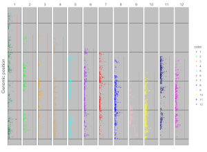
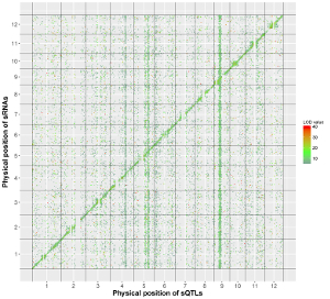
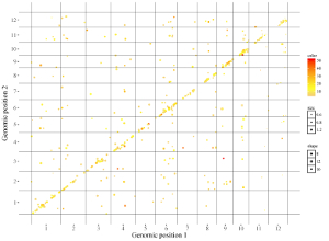
2. Two-genome plot

2.1 Data of genome along the horizontal axis

The dataset should contain only 2 columns with fixed order. Column names are optional.
1st column: chromosome ID.
2nd column: chromosome length.

Acceptable input data format can be

 chr     size
   1 43268879
   2 35930381
   3 36406689

or

1   43268879
2   35930381
3   36406689

2.2 Data of genome along the vertical axis

The dataset should contain only 2 columns with fixed order. Column names are optional.
1st column: chromosome ID.
2nd column: chromosome length.

Acceptable input data format can be

   chr     size
 Chr01 41185095
 Chr02 34608401
 Chr03 37032663

or

Chr01   41185095
Chr02   34608401
Chr03   37032663

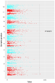
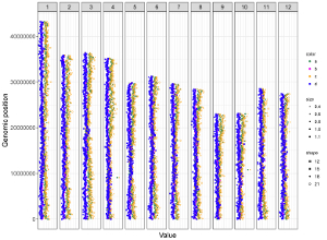
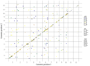
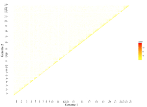
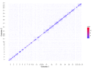
2.3 Point

The dataset should contain >=4 columns.
In the simplest situation, the dataset should contain 4 columns with fixed order. In this case, column names are optional.
1st column: chromosome ID of genome along the horizontal axis.
2nd column: chromosome position in genome along the horizontal axis.
3rd column: chromosome ID of genome along the horizontal axis.
4th column: chromosome position in genome along the vertical axis.

Acceptable input data format can be

 chrX     posX chrY     posY
    4 23006000    6 27706220
    6 26269000    6 27706227
   11 17015000    6 27706228

or

 4  23006000    6   27706220
 6  26269000    6   27706227
11  17015000    6   27706228

To control the color of points, add a color column. In this case, column names are compulsory. The name of the first four columns can be any appropriate variable names in R and the order of the first four columns must be fixed as the simplest situation. The name of the color column must be 'color'. The color column can be a character vector or a numeric vector. If the color column is a character vector, choose the point_discrete plot type.

 chrX     posX chrY     posY color
    1 15414550    1 17415683     a
    1  2314068    1  2291659     a
    1  2583523    1  2546654     c

If the color column is a numeric vector, choose the point_gradual plot type.

 chrX     posX chrY     posY  color
    4 23006000    6 27706220  5.222
    6 26269000    6 27706227 10.424
   11 17015000    6 27706228  5.802

To control the symbol used for each point, add a shape column. Check http://www.endmemo.com/program/R/pchsymbols.php for more information. In this case, column names are compulsory. The name of the first four columns can be any appropriate variable names in R and the order of the first four columns must be fixed as the simplest situation. The name of the shape column must be 'shape'. The shape column should be an integer vector.

 chrX     posX chrY     posY shape
    1 15414550    1 17415683    12
    1  2314068    1  2291659    12
    1  2583523    1  2546654    12

To control the size of each point, add a size column. Larger number in the size column means lareger point size. In this case, column names are compulsory. The name of the first four columns can be any appropriate variable names in R and the order of the first four columns must be fixed as the simplest situation. The name of the size column must be 'size'. The size column should be an integer vector.

 chrX     posX chrY     posY size
    1 15414550    1 17415683  1.2
    1  2314068    1  2291659  1.2
    1  2583523    1  2546654  1.2

Acceptable input data can also be

 chrX     posX chrY     posY color shape
    1 15414550    1 17415683     a    12
    1  2314068    1  2291659     a    12
    1  2583523    1  2546654     c    12

or

 chrX     posX chrY     posY color size
    1 15414550    1 17415683     a  1.2
    1  2314068    1  2291659     a  1.2
    1  2583523    1  2546654     c  1.2

or

 chrX     posX chrY     posY shape size
    1 15414550    1 17415683    12  1.2
    1  2314068    1  2291659    12  1.2
    1  2583523    1  2546654    12  1.2

or

 chrX     posX chrY     posY color shape size
    1 15414550    1 17415683     a    12  1.2
    1  2314068    1  2291659     a    12  1.2
    1  2583523    1  2546654     c    12  1.2

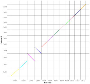
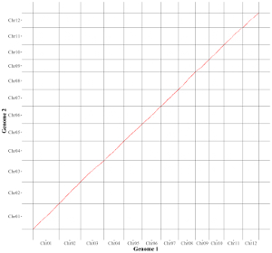
2.4 Segment

The dataset should contain >=6 columns.
In the simplest situation, the dataset should contain 6 columns with fixed order. In this case, column names are optional.
1st column: chromosome ID of genome along the horizontal axis.
2nd column: X-axis start coordinate of segments.
3rd column: X-axis end coordinate of segments.
4th column: chromosome ID of genome along the vertical axis.
5th column: Y-axis start coordinate of segments.
6th column: Y-axis end coordinate of segments.

Acceptable input data can be

  chrX startX stopX  chrY startY stopY
 Chr01    101 21963 Chr01  19600 41490
 Chr01  25221 49370 Chr01  41483 65682
 Chr01  49604 67964 Chr01  65681 84044

or

Chr01     101   21963   Chr01   19600   41490
Chr01   25221   49370   Chr01   41483   65682
Chr01   49604   67964   Chr01   65681   84044

To control the color of segments, add a color column to categorize data into different groups. Then different colors will be assigned to different groups of data. In this case, column names are compulsory. The name of the first six columns can be any appropriate variable names in R and the order of the first six columns must be fixed as the simplest situation. The name of the color column must be 'color'.

  chrX   startX    stopX  chrY   startY    stopY color
 Chr01        1 35619588 Chr01        1 36185095     a
 Chr02 35140161        1 Chr02 34608401        1     b
 Chr03        1 33736842 Chr03 37032663        1     c

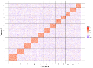
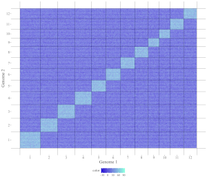
2.5 Rect

The dataset should contain 7 columns with fixed order. Column names are optional.
1st column: chromosome ID of genome along the horizontal axis.
2nd column: X-axis start coordinate of rects.
3rd column: X-axis end coordinate of rects.
4th column: chromosome ID of genome along the vertical axis.
5th column: Y-axis start coordinate of rects.
6th column: Y-axis end coordinate of rects.
7th column: the color of rects.

The 7th column can be a character vector or a numeric vector. For a character vector, choose the rect_discrete plot type. For a numeric vector, choose the rect_gradual plot type.

Acceptable input data format can be

 chrx startx   stopx chry  starty   stopy color
    1      1 1000000    1       1 1000000    41
    1      1 1000000    1 1000001 2000000    43
    1      1 1000000    1 2000001 3000000    59

or

 chrx startx   stopx chry  starty   stopy color
    1      1 1000000    1       1 1000000     b
    1      1 1000000    1 1000001 2000000     b
    1      1 1000000    1 2000001 3000000     b

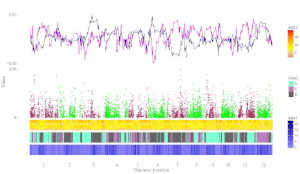
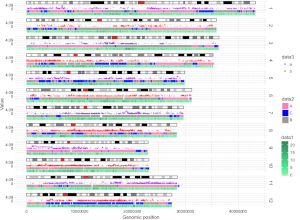
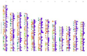
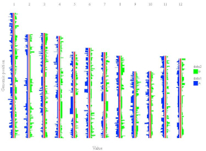
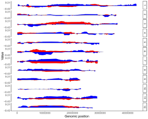
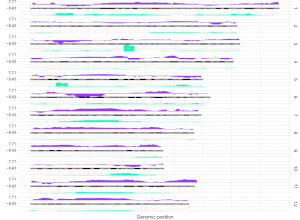
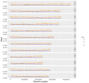
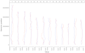
shinyChromosome is a graphical user interface for interactive creation of non-circular whole genome diagrams developed using the R Shiny package.

To create single-genome plot by aligning genome data along all chromosomes of a single genome, go to the Single-genome plot menu.

To cretae two-genome plot for comparison of data across two genomes, go to the Two-genome plot menu.

For the detail format of input data, check the Input data format submenu of the Help menu.

Citation

Yu Y⁺, Yao W^+✉, Wang Y, Huang F. shinyChromosome: An R/Shiny Application for Interactive Creation of Non-circular Plots of Whole Genomes. Genomics, Proteomics & Bioinformatics, 2020 (⁺ co-first author)

Software references

1. R Development Core Team. R: A Language and Environment for Statistical Computing. R Foundation for Statistical Computing, Vienna. R version 3.5.0 (2018)
   
2. RStudio and Inc. shiny: Web Application Framework for R. R package version 1.0.5 (2017)
   
3. Lionel Henry and Hadley Wickham. rlang: Functions for Base Types and Core R and “Tidyverse” Features. R package version 0.2.1 (2018)
   
4. H. Wickham. ggplot2: Create Elegant Data Visualisations Using the Grammar of Graphics. R package version 3.0.0 (2018)
   
5. Gábor Csárdi, Kuba Podgórski, Rich Geldreich. zip: Cross-Platform zip Compression. R package version 2.0.2 (2019)
   
6. Erich Neuwirth. RColorBrewer: ColorBrewer palettes. R package version 1.1-2 (2014)
   
7. Hadley Wickham. plyr: Tools for Splitting, Applying and Combining Data. R package version 1.8.4 (2016)
   
8. Jeffrey B. Arnold. ggthemes: Extra Themes, Scales and Geoms for “ggplot2”. R package version 3.4.0 (2017)
   
9. Christoph Burow, Urs Tilmann Wolpert and Sebastian Kreutzer. RLumShiny: “Shiny” Applications for the R Package “Luminescence”. R package version 0.2.0 (2017)
   
10. Baptiste Auguie. gridExtra: Miscellaneous Functions for “Grid” Graphics. R package version 2.3 (2017)
    
11. Hadley Wickham. reshape2: Flexibly Reshape Data: A Reboot of the Reshape Package. R package version 1.4.3 (2017)
    
12. Matt Dowle and Arun Srinivasan. data.table: Extension of “data.frame”. R package version 1.10.4-3 (2017)
    
13. JJ Allaire, Jeffrey Horner, Vicent Marti and Natacha Porte. markdown: “Markdown” Rendering for R. R package version 0.8 (2017)
    

Further references

This application was created by Yiming Yu and Wen Yao. Please send bugs and feature requests to Yiming Yu (yimingyyu at gmail.com) or Wen Yao (venyao at qq.com). This application uses the shiny package from RStudio.

Note

For Mac users, we recommend using shinyChromosome with the Google Chrome browser or other browsers developed based on Chrominum.